

SQL stands for Structured Query Language. It is a programming language primarily used for managing data held in a relational database management system.
The main functions of SQL can be summarised using the acronym CRUD:
- Create: Adding new records (data).
- Read: Querying and retrieving existing records.
- Update: Modifying existing records.
- Delete: Removing records.
Why Learn SQL?
You might wonder why in the age of chat bots and easy to use spreadsheets why I would recommend you learn SQL. Well, there are many reasons, but the biggest are:
For makers
- Sensor Logging: An ESP32 or Pi sending temperature, humidity or air quality readings every minute soon fills a CSV that no spreadsheet wants to open. Put it in SQLite and “the average for each hour while the laser was running” is one query.
- Home Assistant: Its history lives in a SQLite database (home-assistant_v2.db). Knowing SQL means you can ask it questions the dashboard can’t answer.
- Parts and Filament Inventory: What you have, where it lives and which project used it is relational data. That is the spreadsheet search-and-replace problem from further down, solved properly.
- Selling What You Make: WordPress and WooCommerce run on MySQL, so your shop’s orders and products are a query away when the built-in reports don’t show what you want.
In general
- Data Logging: Anyone who has had to search, sort, slice and dice a large log file knows the pain. Being able to just get back the information you are interested in feels like a super power after that.
- Job Opportunities: SQL skills can significantly enhance your job prospects, and not just in data-specific roles. These skills allow you to see data differently, both in terms of retrieval of actual data and also conceptually.
- Data Management and Reporting: SQL allows you to handle and manipulate large quantities of complex and inter-related data efficiently in ways that are much more difficult to do with other tools.
- Cross-Platform: The basics of SQL carry over to other database management systems (DBMS), such as MySQL, Microsoft SQL Server and Oracle.
Practise along:
Open makerhacks.com/sql-fiddle, press Execute, and the coffee shop tables are ready to query.
Understanding Databases
At its core, a database is a structured collection of data. You can think of it as a digital filing system, similar to an Excel spreadsheet with columns (fields) and rows (records). While Excel is great for small amounts of data, databases are designed to handle larger and more complex sets of information.
Types of Databases
There are two primary types of databases to be aware of:
- Relational Databases: This type involves tables with relationships between them. For example, in a coffee shop database, you might have separate tables for customers, orders, and products, all linked together.
- Non-relational Databases: These do not use structured tables. They might be used for unstructured data like documents or records. An example is NoSQL databases.
Advantages of Relational Databases
Consider the roadblocks that form when using only spreadsheets and your data becomes more than simple lists of things. For example you might start to categorise, and then want to change the categories. With a spreadsheet that means doing a search and replace across all your sheets, and it can lead to data entry mistakes, for example “beans” versus “bean”.
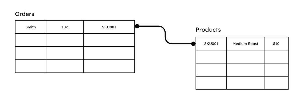
Another issue with spreadsheets is if you have a product code or SKU and the written description, price, stock levels etc it wouldn’t make sense to keep all of that in a single sheet, even using VLOOKUP and such can get cumbersome.
In a relational database, you can query the data you need via the relations or connections between various tables, in a way that gives you just what you need, quickly.
Database Management Systems (DBMS)
Lots of different DBMS are available. Some popular options include:
- MySQL: A free, open-source DBMS widely used for web applications.
- Microsoft SQL Server: A proprietary DBMS for enterprise applications.
- Oracle Database: A multi-model database management system with high license fees.
- SQLite: Free database stored as a single file that can be easily copied from machine to machine.
Regardless of the system, all of them use broadly the same SQL to perform operations.
Getting Started with SQL
To start using SQL, you’ll follow these steps to create a database, add tables, and manage data. Many web hosts set up a DBMS for you by default or have a one-click setup option. If not, setting up a DBMS is relatively straightforward but outside the scope of this guide.
Step 1: Create a Database
Start by creating a database. Think of it as the box that everything else is going to go into. It is empty until you add tables to it:
CREATE DATABASE my_database_name;
Step 2: Create a Table
After creating a database, the next step is to create a table. For instance, if you are creating a coffee shop database, the command would look like this:
CREATE TABLE coffee (
    id INT PRIMARY KEY,
    name VARCHAR(255),
    region VARCHAR(255),
    roast VARCHAR(255)
);
An INT is a whole number, and VARCHAR(255) is text that can’t be any longer than 255 characters.
You could use a type that holds as much text as you like, so why limit it? Efficiency.
The more relaxed we are about what goes in, the slower everything gets. For your Magic: The Gathering cards it won’t matter, because there are never going to be millions of records.
Think, though, about a large organisation with thousands of customers, who all have orders and payments and subscriptions, and it soon gets really big. Being strict at the start gives you an easier life as things grow.
We have already been a bit lazy here, though. Why is region something you type in? A list of regions already exists in the world. And how many roasts are there going to be? Dark, medium, light.
That is the difference between spreadsheets and databases. For every column, ask whether it is free text that belongs to this one record, like a description, or is it a category that deserves its own table. I am keeping it sloppy for this guide, but sorting things into categories and linking them up is what saves you time later.
On naming: I keep table and column names lower case with underscores between the words, like coffee_id. A hyphen can be read as a minus sign and a space means quoting the name every time you use it. If names are always lower case with underscores, you never have to remember which letters were capitals.
Step 3: Insert Data
To add data to your table, you can use the INSERT command:
INSERT INTO coffee (id, name, region, roast)
VALUES (1, 'Default Roast', 'Ethiopia', 'Light');
You tell it the columns you are inserting into, then the values, in the same order. To add several rows at once, separate each set of values with a comma.
A lot of the time the data will arrive as a CSV file (comma separated values) and you run an import. The thing to watch is quote marks. Text values are wrapped in single quotes, so anything with an apostrophe in it, a plural or an Irish surname, ends the text early and breaks the query. Double the apostrophe to get it through:
INSERT INTO coffee (id, name, region, roast)
VALUES (11, 'Barista''s Choice', 'Peru', 'Medium');
Step 4: Query Data
You can retrieve data using the SELECT command:
SELECT * FROM coffee;
The star means every column. You get the whole table back, in id order.
Sorting and Choosing Columns
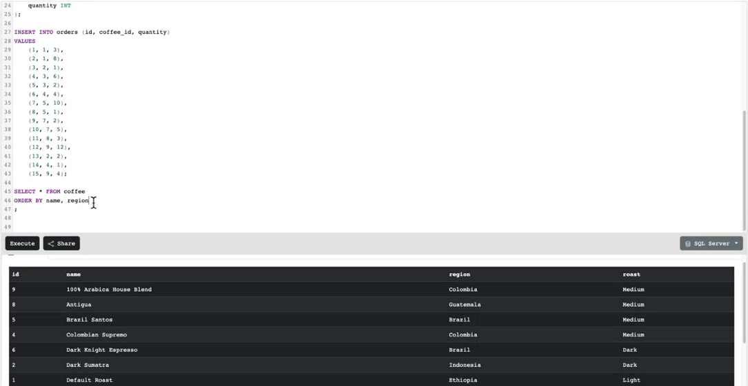
You can sort by any column, and DESC turns it upside down:
SELECT * FROM coffee ORDER BY region;
SELECT * FROM coffee ORDER BY id DESC;
And you can ask for only the columns you want, by naming them in place of the star:
SELECT name, region FROM coffee ORDER BY region;
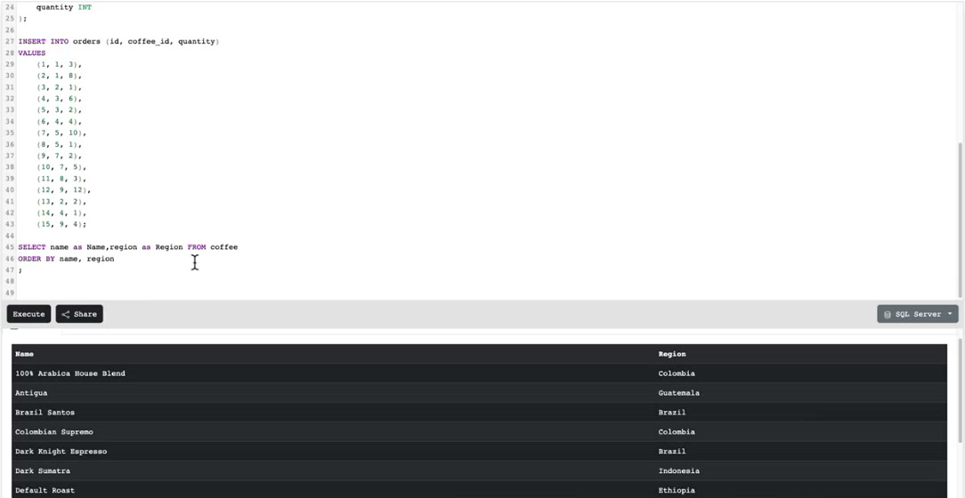
So far this is all stuff you could do in a spreadsheet.
Filtering with WHERE
WHERE narrows the rows down. Only the coffees from Brazil:
SELECT * FROM coffee WHERE region = 'Brazil';
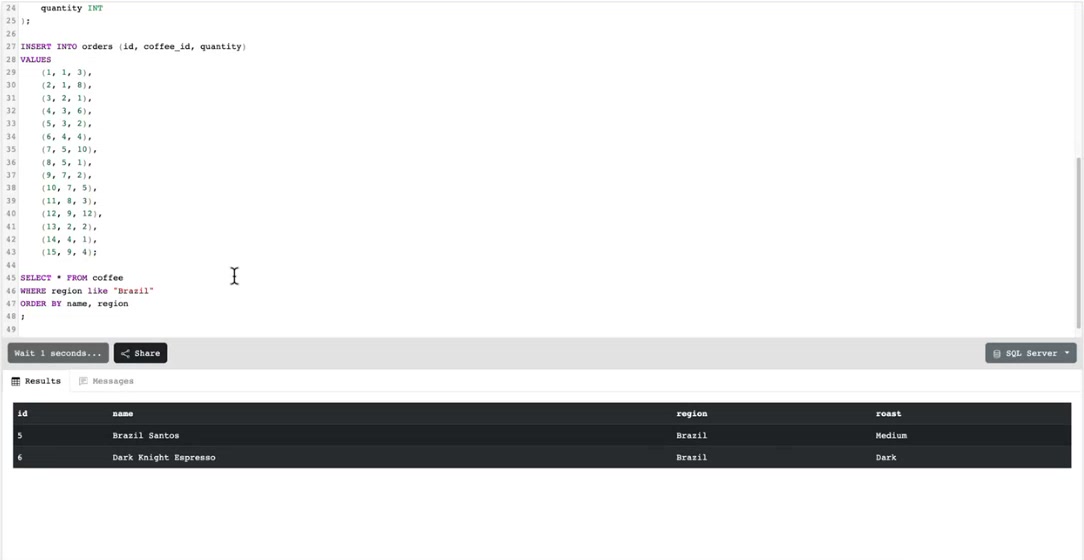
That returns two, Brazil Santos and Dark Knight Espresso. You can also compare numbers, which works on dates too:
SELECT * FROM coffee WHERE id > 4;
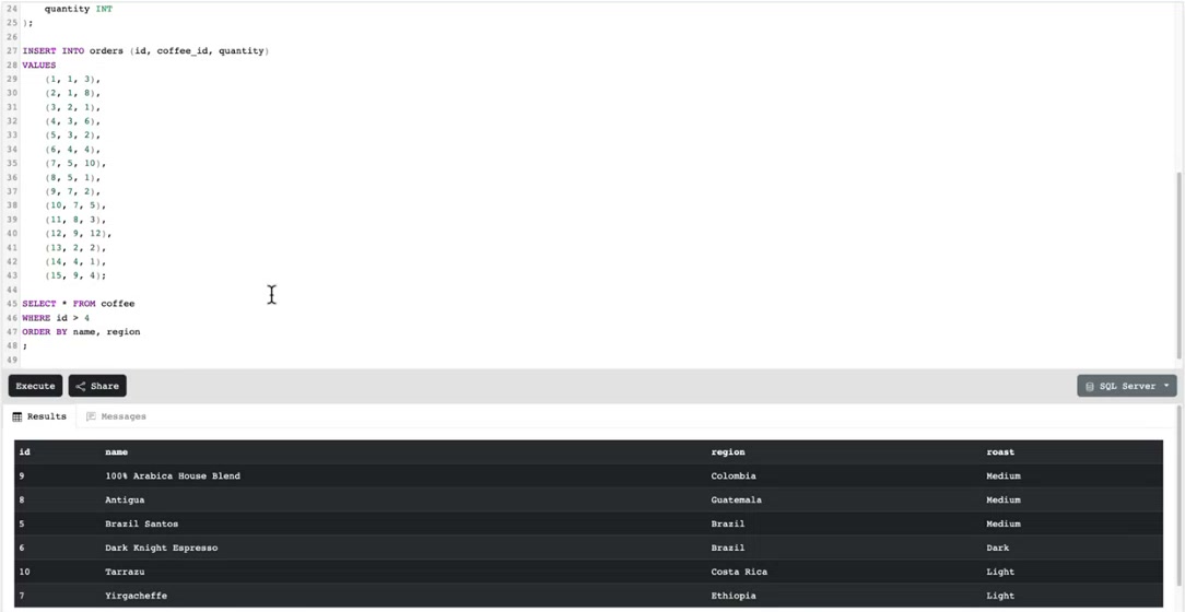
When you are not sure of the exact text, use LIKE. A percent sign stands for any number of characters and an underscore stands for exactly one:
SELECT * FROM coffee WHERE region LIKE 'B%';
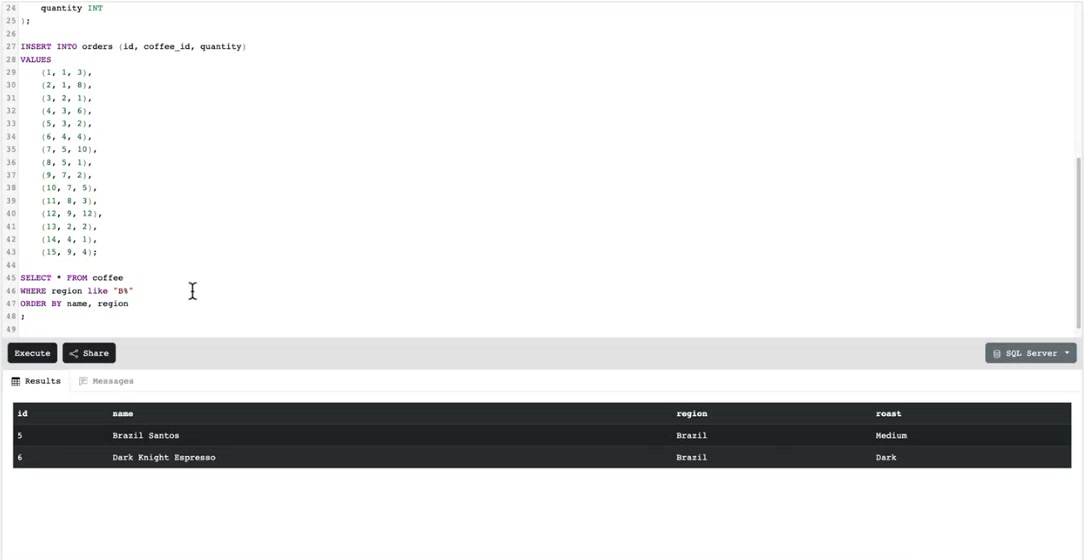
That is every region starting with a B. It is handy for names, because my surname has two Rs and two Ts and not everybody spells it that way, and for finding everyone with an email address at one company with LIKE '%@example.com'.
Step 5: Update Records
If you need to change existing records, use the UPDATE command:
UPDATE coffee SET roast = 'Dark' WHERE id = 1;
It is pretty much English: update this table, set this column to this value, where the id is 1.
This is where unique id numbers earn their keep. If I rename Default Roast, anything that looked it up by name won’t find it any more, but id 1 is still id 1. It is the same with people. If I change from a personal email address to a work one and everything was matched on email address, the system thinks I am a different person.
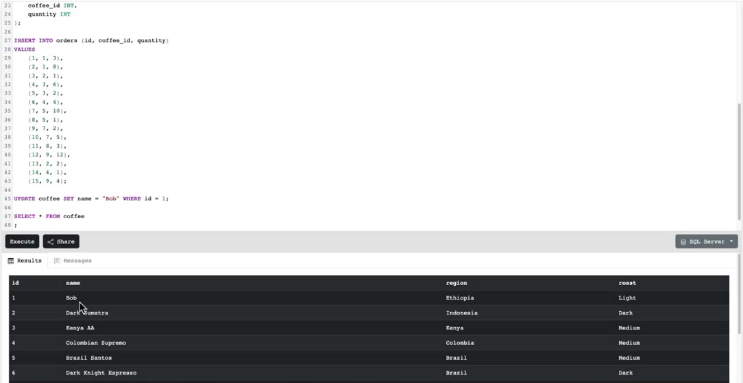
You don’t have to use the id. This changes every light roast in one go:
UPDATE coffee SET roast = 'Weak' WHERE roast = 'Light';
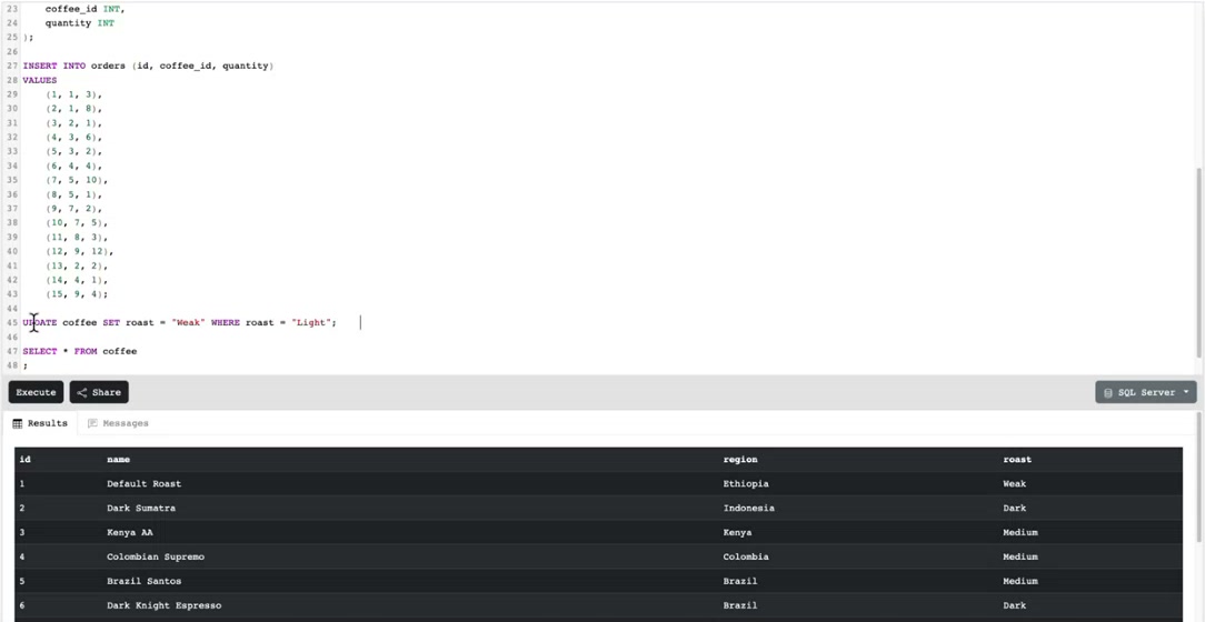
That is powerful, and it is also a massive bomb blast across your data if the WHERE is wrong, or missing. Leave the WHERE off and every row is changed. So do a SELECT first with the same WHERE, read back what you are about to change, and spot check it.
Step 6: Delete Records
To remove records from a table, use the DELETE command:
DELETE FROM coffee WHERE id = 1;
If we missed off the WHERE id = 1, it would delete everything. If the WHERE is a bit fuzzy, say LIKE 'A%', it deletes everything starting with an A. It doesn’t complain and it doesn’t ask if you are sure. It says OK and they are gone.
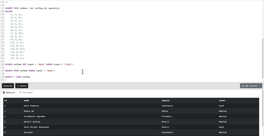
In a business system you often don’t delete at all. A shop would not normally delete a product. It would set the stock level to zero, or have a column that says the product is no longer in use, because ten years of orders, receipts and invoices all point at that product. Delete the red widget and every one of them has a hole in it, and your accountant will be cross.
The same goes for something like a membership. You mark it as ended. If you deleted it, you could never answer how many members you had last year. The database will happily let you do it, but that doesn’t make it the right thing to do.
NULL Is Not the Same as Blank
If a row is added with a value missing, that column holds NULL. NULL isn’t zero and it isn’t an empty piece of text. It means there is no value at all, and it catches everybody out, because nothing is ever equal to NULL. This returns no rows, even when some roasts are missing:
SELECT * FROM coffee WHERE roast = NULL;
You have to ask for it by name:
SELECT * FROM coffee WHERE roast IS NULL;
It shows up most when you import data or move it between systems, where one system left a field empty and the other expected something. It goes back to the sloppiness: the stricter you are at the start, the fewer of these you have to hunt down.
Multi-Table Queries with WHERE and JOINs
This is where the relational part really kicks in. Everything so far has been CRUD on one table. Joining tables together is one of the most powerful things a relational database does. In Excel the nearest you get is a VLOOKUP into another tab.
The playground has a second table, orders, for mail orders of bags of coffee:
CREATE TABLE orders (
    id INT PRIMARY KEY,
    coffee_id INT,
    quantity INT
);
Notice it is all numbers: the order id, which coffee was ordered, and how many bags. A real one would have a date and a customer id as well. There are 15 orders in there, and on their own they are meaningless. Order 1 was three bags of coffee 1. The join is what turns coffee 1 back into Default Roast.
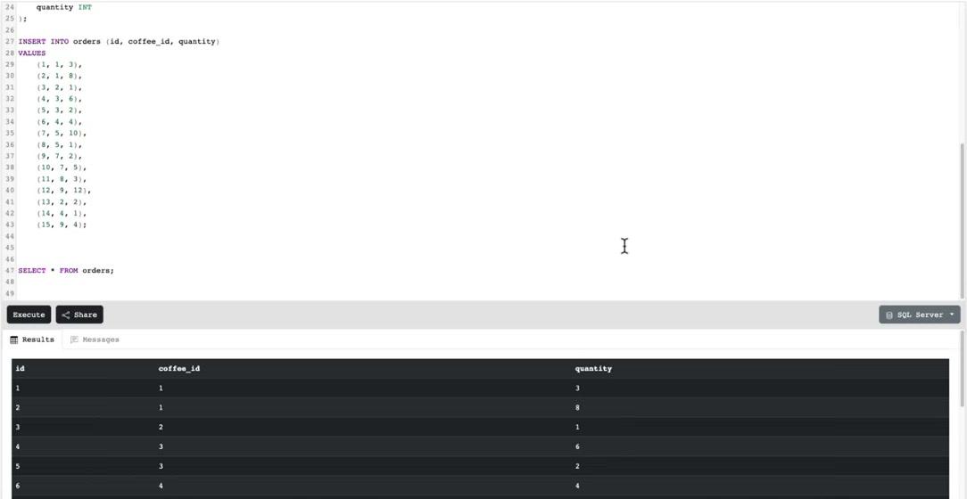
The JOIN clause is used to combine rows from two or more tables, based on a related column between them.
Here are the different types of JOINs in SQL:
(INNER) JOIN: Returns only rows that have matching values in both tablesLEFT (OUTER) JOIN: Returns all rows from the left table, and only the matched rows from the right tableRIGHT (OUTER) JOIN: Returns all rows from the right table, and only the matched rows from the left tableFULL (OUTER) JOIN: Returns all rows when there is a match in either the left or right table
Joining Tables with WHERE
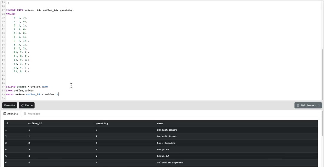
Before the JOIN keyword existed, tables were joined by listing them all after FROM and matching them up in the WHERE clause. To see each order with the name of the coffee:
SELECT orders.id, orders.quantity, coffee.name
FROM orders, coffee
WHERE orders.coffee_id = coffee.id;
That returns all 15 orders, each with its coffee name, and you will still see this style in older code.
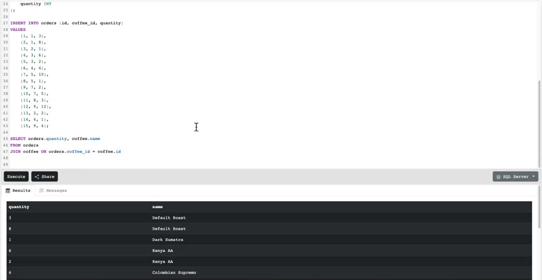
Joining Tables with INNER JOIN
SELECT orders.id, orders.quantity, coffee.name
FROM orders
INNER JOIN coffee ON orders.coffee_id = coffee.id;
This returns the same 15 rows. The difference is that the matching condition is in the ON clause, next to the table it connects, rather than in the WHERE clause with any filters.
Why Use JOIN Instead of WHERE?
- Joins and filters are kept separate. ON says how the tables are connected and WHERE says which rows you want, so adding a filter does not make the query harder to read:
SELECT orders.id, orders.quantity, coffee.name
FROM orders
INNER JOIN coffee ON orders.coffee_id = coffee.id
WHERE coffee.roast = 'Dark';
- A missing condition causes an error. If you leave the WHERE off the comma version, the database matches every order with every coffee. That is 15 orders times 10 coffees, so 150 rows, and no error. A JOIN without its ON clause is a syntax error in most databases, so the mistake is caught.
- Some joins can only be written this way. LEFT, RIGHT and FULL joins have no standard WHERE equivalent. SQL Server used to have a
*=shortcut for it, and it was removed years ago. - Larger queries are easier to follow. With three or four tables, each JOIN line has its own condition, so you can see how the tables are connected.
Keeping Unmatched Rows with LEFT JOIN
An INNER JOIN only returns rows that match in both tables. A LEFT JOIN keeps every row from the first (left) table, matched or not:
SELECT coffee.name, orders.quantity
FROM coffee
LEFT JOIN orders ON orders.coffee_id = coffee.id;
This returns every coffee. Coffees with orders are listed once per order, and Dark Knight Espresso and Tarrazu, which have no orders, are listed with NULL in the quantity column. Add a WHERE to keep only those, and you have a list of coffees that aren’t selling:
SELECT coffee.name
FROM coffee
LEFT JOIN orders ON orders.coffee_id = coffee.id
WHERE orders.id IS NULL;
Aggregate Functions and GROUP BY
The queries so far have returned rows as they are stored. Aggregate functions calculate a single value, for example a count or a total, from many rows.
Common Aggregate Functions
| Function | What it gives you |
|---|---|
COUNT(*) | How many rows |
SUM(column) | The total |
AVG(column) | The average |
MIN(column) | The smallest value |
MAX(column) | The largest value |
You can use several at once:
SELECT
    COUNT(*) AS total_orders,
    SUM(quantity) AS total_bags,
    AVG(quantity) AS average_bags,
    MIN(quantity) AS smallest_order,
    MAX(quantity) AS biggest_order
FROM orders;
That gives one row: 15 orders, 64 bags, an average of about 4.27, the smallest order 1 bag and the biggest 12. The AS part names each column in the result, otherwise you get headings like SUM(quantity) or no heading at all.
Note that SQL Server returns 4 here, not 4.27. Because quantity is a whole number column, SQL Server calculates the average as a whole number, while MySQL returns the decimals. Multiply by 1.0 to get the decimals in SQL Server:
SELECT AVG(quantity * 1.0) AS average_bags FROM orders;
Grouping Results with GROUP BY
On its own an aggregate gives one answer for the whole table. GROUP BY splits the rows into groups first and gives you one answer per group. How many coffees of each roast?
SELECT roast, COUNT(*) AS coffees
FROM coffee
GROUP BY roast;
Dark 2, Light 3, Medium 5.
GROUP BY is often combined with a join. This query shows the number of orders and bags for each coffee, with the best sellers first:
SELECT coffee.name, COUNT(orders.id) AS orders, SUM(orders.quantity) AS bags
FROM coffee
INNER JOIN orders ON orders.coffee_id = coffee.id
GROUP BY coffee.name
ORDER BY bags DESC;
The 100% Arabica House Blend has the most, with 16 bags, followed by Default Roast and Brazil Santos with 11 each.
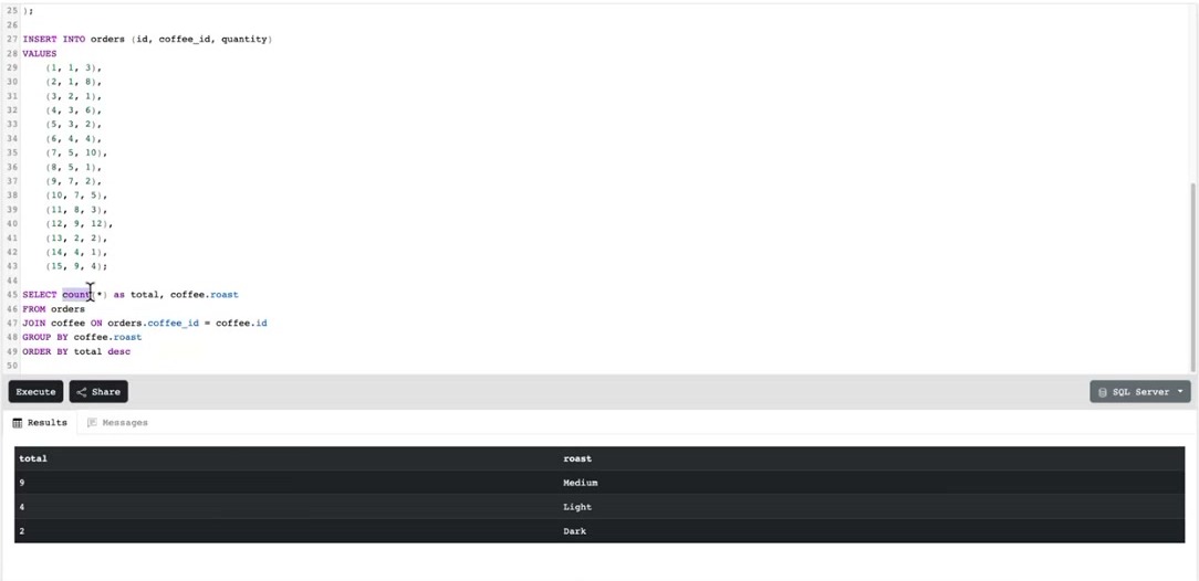
Every column in the SELECT must either be inside an aggregate function or be listed in the GROUP BY. Ask for coffee.region in the query above without grouping by it, and SQL Server refuses. Current versions of MySQL also return an error. Older versions picked a value from the group without warning you, which could give wrong results.
Filtering with WHERE and HAVING
WHERE filters rows before they are grouped. HAVING filters the groups afterwards, so it is the one to use when the condition is about a total. Coffees that have sold at least 10 bags:
SELECT coffee.name, SUM(orders.quantity) AS bags
FROM coffee
INNER JOIN orders ON orders.coffee_id = coffee.id
GROUP BY coffee.name
HAVING SUM(orders.quantity) >= 10
ORDER BY bags DESC;
Three coffees meet the condition, the House Blend, Default Roast and Brazil Santos.
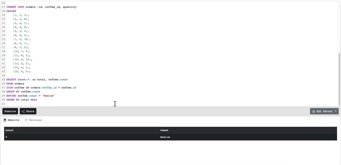
Repeat the SUM(...) in HAVING rather than using the bags name. MySQL lets you use the name there, but SQL Server doesn’t, so writing it out works on both.
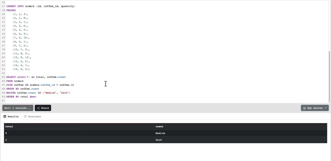
You can use both in one query. Bags per region, leaving out dark roasts:
SELECT coffee.region, SUM(orders.quantity) AS bags
FROM coffee
INNER JOIN orders ON orders.coffee_id = coffee.id
WHERE coffee.roast <> 'Dark'
GROUP BY coffee.region
ORDER BY bags DESC;
Counting Rows vs Counting Values
COUNT(*) counts rows. COUNT(column) counts only the rows where that column is not NULL. That matters with a LEFT JOIN:
SELECT coffee.name, COUNT(*) AS row_count, COUNT(orders.id) AS order_count
FROM coffee
LEFT JOIN orders ON orders.coffee_id = coffee.id
GROUP BY coffee.name;
Dark Knight Espresso and Tarrazu show a row count of 1 but an order count of 0. The LEFT JOIN still gives them a row, just one full of NULLs, so COUNT(*) would wrongly report one order each.
Sub Queries and Querying Queries
A subquery is a SELECT inside another query. The inner query runs first, and the outer query uses its result. This lets you answer a question with one query instead of running two and copying the results between them.
Nested Selects with IN
Which coffees have had a big order? The inner query finds the coffee ids from orders of more than five bags, and the outer query looks up their names:
SELECT name
FROM coffee
WHERE id IN (
    SELECT coffee_id FROM orders WHERE quantity > 5
);
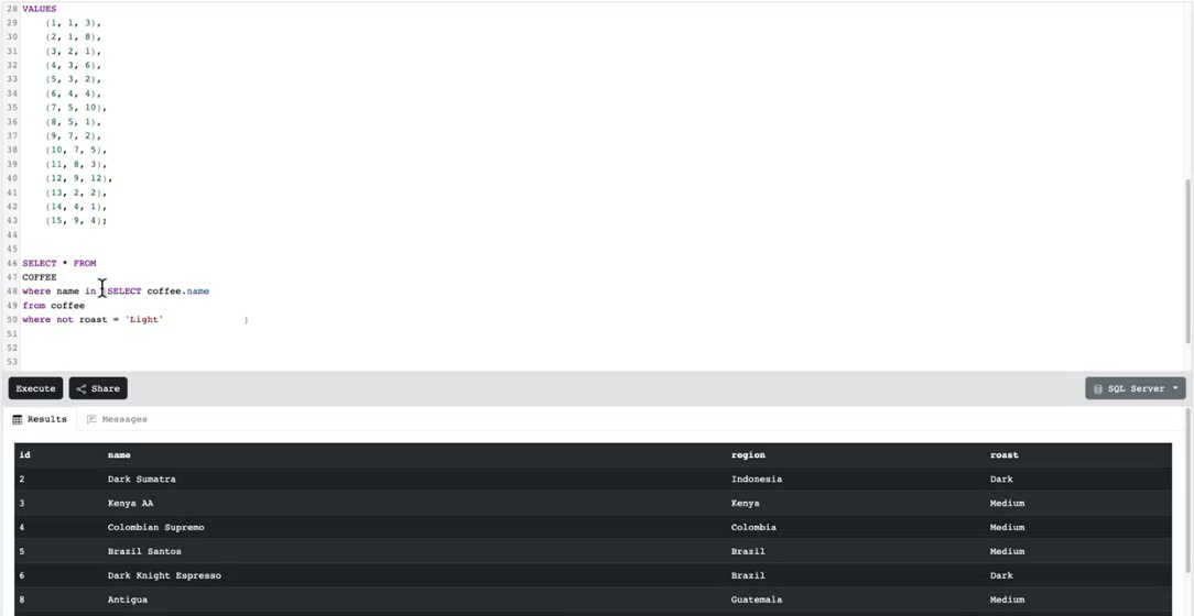
Flip it with NOT IN to find coffees nobody has ordered:
SELECT name
FROM coffee
WHERE id NOT IN (SELECT coffee_id FROM orders);
Be careful with NULLs. If the subquery returns a NULL value, NOT IN returns no rows at all. NOT EXISTS does not have this problem, so it is the safer choice:
SELECT name
FROM coffee c
WHERE NOT EXISTS (
    SELECT 1 FROM orders o WHERE o.coffee_id = c.id
);
Comparing Against a Single Value
When the inner query returns exactly one value, you can use it anywhere you would type a number. Here, orders bigger than the average order:
SELECT id, quantity
FROM orders
WHERE quantity > (SELECT AVG(quantity) FROM orders);
Subqueries in the FROM Clause
You can also put a whole query in the FROM clause and treat its result as if it were a table. This is useful when you need to filter on a calculated value, such as a total:
SELECT region, total_bags
FROM (
    SELECT c.region, SUM(o.quantity) AS total_bags
    FROM coffee c
    JOIN orders o ON o.coffee_id = c.id
    GROUP BY c.region
) AS region_totals
WHERE total_bags > 5;
The inner query adds up the bags ordered per region, and the outer one keeps only the regions over five. The AS region_totals name is required. Both MySQL and SQL Server return an error for a subquery in FROM without a name.
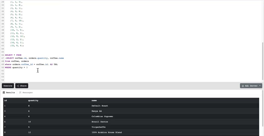
Subqueries can be confusing to read, but sometimes they are the only way to do it. A past client was a chain of pubs with very different types of pub, from family pubs with adventure playgrounds all the way through to posh gastro pubs where kids were pretty much not allowed. We had to build a “find my nearest” search with checkboxes: it needs a playground, it needs car parking, and so on. Nearest meant looking up where the person was and using Pythagoras to work out the distance to every pub as the crow flies.
The catch was that we were never allowed to return nothing. They didn’t want it to say no pubs match your criteria. So each checkbox became a subquery that gave the pub a score, and the results were ordered by the score. Even if the top pub didn’t have everything you asked for, you always got a list back. And it all had to be fast, because otherwise people get bored and click away.
Saving a Query as a View
If you find yourself writing the same big join again and again, you can save it as a view. A view is like a virtual table. It holds no data of its own. Each time you select from it, the saved query runs and you query the result:
CREATE VIEW order_details AS
SELECT orders.id, orders.quantity, coffee.name, coffee.region, coffee.roast
FROM orders
INNER JOIN coffee ON orders.coffee_id = coffee.id;

SELECT name, quantity FROM order_details WHERE roast = 'Medium';
I once worked on a holiday cottage site where every cottage sat in a town, in a county, in a region, in a country. Getting a full address meant one massive join, so that join became a view and everything else selected from it.
MySQL vs Microsoft SQL Server Syntax Differences
Everything above works on both MySQL and SQL Server. Beyond the basics, each has its own version of SQL, and these are the differences you are most likely to come across when moving between them.
| What | MySQL | SQL Server (T-SQL) |
|---|---|---|
| Quoting a table or column name | `order` (backticks) | [order] (square brackets) |
| Text values | 'text' (also "text" by default) | 'text', and N'text' for Unicode |
| Limit the number of rows | SELECT ... LIMIT 10 | SELECT TOP 10 ... |
| Join text together | CONCAT(a, b) | a + b or CONCAT(a, b) |
| Auto-numbered ids | AUTO_INCREMENT | IDENTITY(1,1) |
| Current date and time | NOW() | GETDATE() |
| Replace NULL with a value | IFNULL(x, 0) | ISNULL(x, 0) |
| True or false column | BOOLEAN (really TINYINT(1)) | BIT |
COALESCE(x, 0) works on both, so it’s the one to use if your code has to run on either.
Quoting Table and Column Names
You only need to quote a name if it clashes with a keyword or contains a space. A column called order is a classic, because ORDER is part of ORDER BY:
-- MySQL
SELECT `order`, `coffee name` FROM orders;

-- SQL Server
SELECT [order], [coffee name] FROM orders;
Standard SQL uses double quotes for names, and both can be set up to accept that, but they behave differently by default. In MySQL, double quotes mean a string unless the ANSI_QUOTES mode is on. The simplest approach is to avoid names that need quoting.
Wildcards and LIKE
Both use % for any number of characters and _ for exactly one, with LIKE:
SELECT name FROM coffee WHERE name LIKE 'Dark%';
SELECT name FROM coffee WHERE region LIKE '_enya';
SQL Server adds square-bracket character sets, which MySQL does not have:
-- SQL Server only: names starting with A, B or C
SELECT name FROM coffee WHERE name LIKE '[ABC]%';

-- SQL Server only: names not starting with A
SELECT name FROM coffee WHERE name LIKE '[^A]%';
In MySQL, use REGEXP instead:
SELECT name FROM coffee WHERE name REGEXP '^[ABC]';
Searching for a literal % or _ is different too. MySQL uses a backslash, SQL Server wraps the character in brackets:
-- MySQL
SELECT name FROM coffee WHERE name LIKE '100\% Arabica%';

-- SQL Server
SELECT name FROM coffee WHERE name LIKE '100[%] Arabica%';
Limiting Results
The most common difference is how you limit the number of rows returned:
-- MySQL: the five biggest orders
SELECT id, quantity FROM orders ORDER BY quantity DESC LIMIT 5;

-- SQL Server: the same thing
SELECT TOP 5 id, quantity FROM orders ORDER BY quantity DESC;
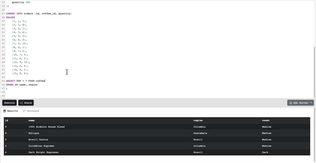
For paging through results, MySQL has LIMIT 5 OFFSET 10, and SQL Server uses OFFSET 10 ROWS FETCH NEXT 5 ROWS ONLY after the ORDER BY.
Mistakes I Commonly Make
I have been writing SQL for a long time and I still get it wrong, especially during demos in front of people. I ran through everything in this guide live for a training session and made most of these within that hour. If you hit the same errors, you are in good company.
Listing Both Tables and Then Joining Anyway
I learned to join tables the old way, with both tables after FROM and the match in the WHERE. So when I write a JOIN, my fingers automatically type both tables first:
SELECT orders.id, orders.quantity, coffee.name
FROM orders, coffee
INNER JOIN coffee ON orders.coffee_id = coffee.id;
That mentions coffee twice and the database complains. Pick one style. With JOIN, only the first table goes after FROM.
Forgetting the Comparison in ON
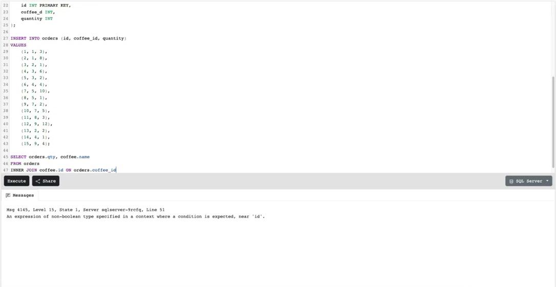
If you write ON orders.coffee_id and stop, SQL Server replies with “An expression of non-boolean type specified in a context where a condition is expected”. In English: ON wants a question it can answer yes or no, so it needs both sides, orders.coffee_id = coffee.id.
Making Up Column Names
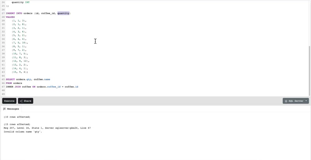
I typed qty. The column is called quantity. The database will not guess. When a query fails, check the names against the table before you look for anything cleverer.
Using a Table That Is Not in the Query
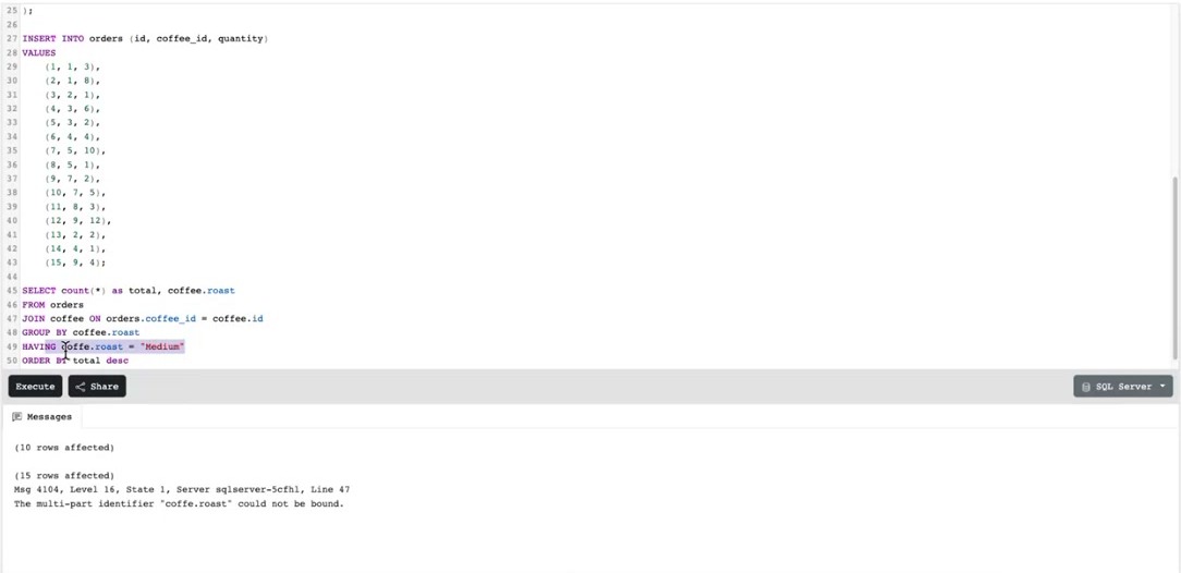
“The multi-part identifier coffee.roast could not be bound” is SQL Server telling you that you asked for coffee.roast but never brought the coffee table into the query. Either join it in, or you have a typo in the table name.
Putting Things in the Wrong Order
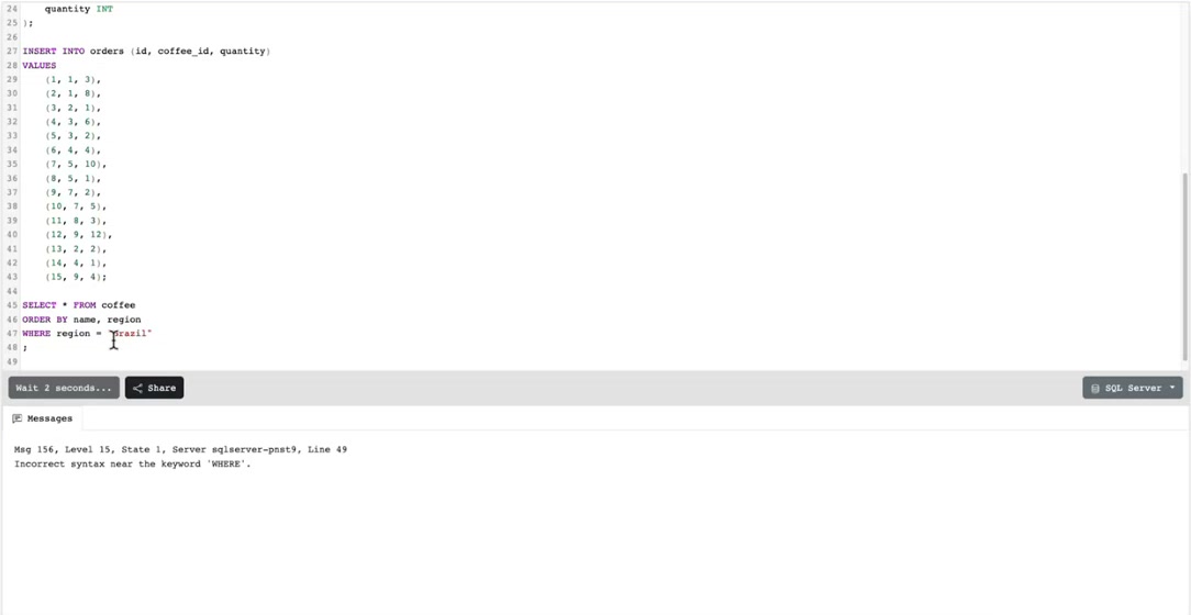
The order of the instructions matters. It is always SELECT, FROM, JOIN, WHERE, GROUP BY, HAVING, ORDER BY. I regularly put an ORDER BY above the WHERE, or try to filter a count with WHERE when it has to be HAVING. WHERE comes first and works on rows. HAVING comes after the grouping and works on the totals.
Selecting a Column I Did Not Group By
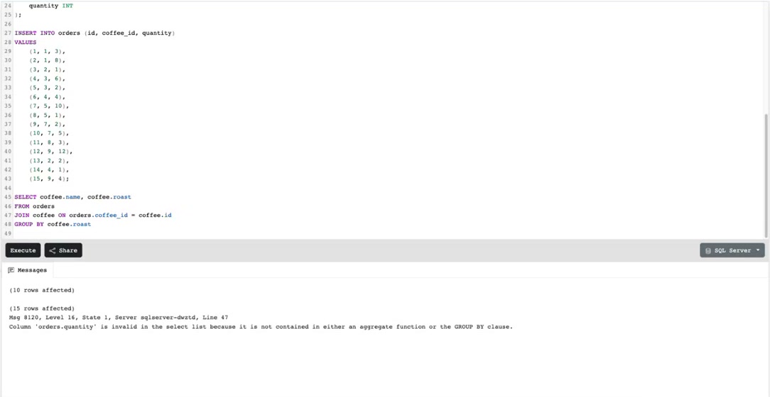
If you group by roast and also ask for the name, the database does not know which name to show for a group of five coffees. Everything in the SELECT has to be in the GROUP BY or inside a function like COUNT. This is the one I walk into every single time.
Using LIMIT on SQL Server
This one hits me a lot when I move between the two. MySQL wants LIMIT 5 at the end, SQL Server wants SELECT TOP 5 at the start. Same idea, different place in the query.
Editing the Wrong Statement
In the playground the whole script runs every time: create the table, insert the rows, then the query. More than once I changed the INSERT when I meant to change the SELECT underneath it, and then wondered why the results looked odd. Check which statement your cursor is in.
UPDATE or DELETE Without a WHERE
Everything above gives you an error message, which is the database being helpful. This one does not. UPDATE coffee SET roast = 'Weak' with no WHERE changes every row, and DELETE FROM coffee empties the table. So run it as a SELECT first:
SELECT * FROM coffee WHERE roast = 'Light';
Read back what you are about to change, and only then swap the SELECT for the UPDATE or DELETE with the same WHERE.

 xTool O1 Omni Review